
We talked earlier about the “graphs” of functions and relations, which were sets of ordered pairs (or triples, or …). As I said, it’s common for theorists to equate functions and relations with these graphs.
What we’re going to talk about now is a mathematical structure that’s also called a “graph,” but with a somewhat different meaning. If I want to be explicit, we can call these new things “graph structures,” though usually we’ll just say “graphs.” There are connections to the sets-of-pairs notion of a graph, but some graphs in one sense wouldn’t be counted as graphs in the other.
Specifically, and anticipating the vocabulary to follow: if you have a binary relation R on a finite domain V (whose set-of-pairs graph would be a subset of V²), that will correspond to a digraph structure whose vertices are V and whose edges are given by R, as long as you allow self-loops in the digraph (ordinarily these are not allowed) or if R is irreflexive. Subject to the same caveats, if R is symmetrical, it will also correspond to a ugraph structure.
See the below section on Graphs and Relations.
A graph is a mathematical structure consisting of (usually at least 1 but in any case) finitely many vertices or nodes, on the one hand, and 0 or more edges joining or connecting two vertices, on the other. There are several variations on this basic idea.
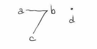
In a simple or undirected graph, the edges have no direction; in directed graphs or digraphs, they do. In the latter case the directed edges are sometimes called arrows or arcs. When I want to talk specifically about undirected graphs, I will say “ugraph,” but this is not standard terminology. When I say “graph,” I mean to be talking about either ugraphs or digraphs. Here are some examples (we’ll explain what it is for a graph to be “unconnected” below, but you can probably already guess).
I’ve used the tags a b and c in these diagrams so that we can refer to the different vertices/positions in the graph. Clearly, for this purpose, different positions should be tagged differently. There is a subtly different practice, though, when we’re using graphs not just to talk about their mathematical structure, but to represent some pre-existing external structure. When we’re doing that, we sometimes want to talk about the objects that occupy the vertices/positions in the graph, that is, that that position in the graph represents. When doing this, it’s not always forbidden that one object simultaneously occupies multiple positions in the graph. For example: suppose that a graph represents train lines, and that United trains and Bellagio trains both run through Market Street Terminal. But passengers are only allowed to transfer for free between trains of the same company. Then we might choose to have Market Street Terminal occupy two vertices in the graph, one where edges representing United train services arrive and depart, and the other representing Bellagio train services. The way mathematicians talk about graphs, they’d say that in this case Market Street Terminal labels two vertices. I think this terminology is really unfortunate, but there it is. We’ll talk about this more below. For the time being, we’re just focusing on the graph structures themselves, without any objects “labeling” the vertices (or on the edges either). My as and bs and so on are just ways to refer to the different graph vertices. They’re not playing the same role as Market Street Terminal in the example.
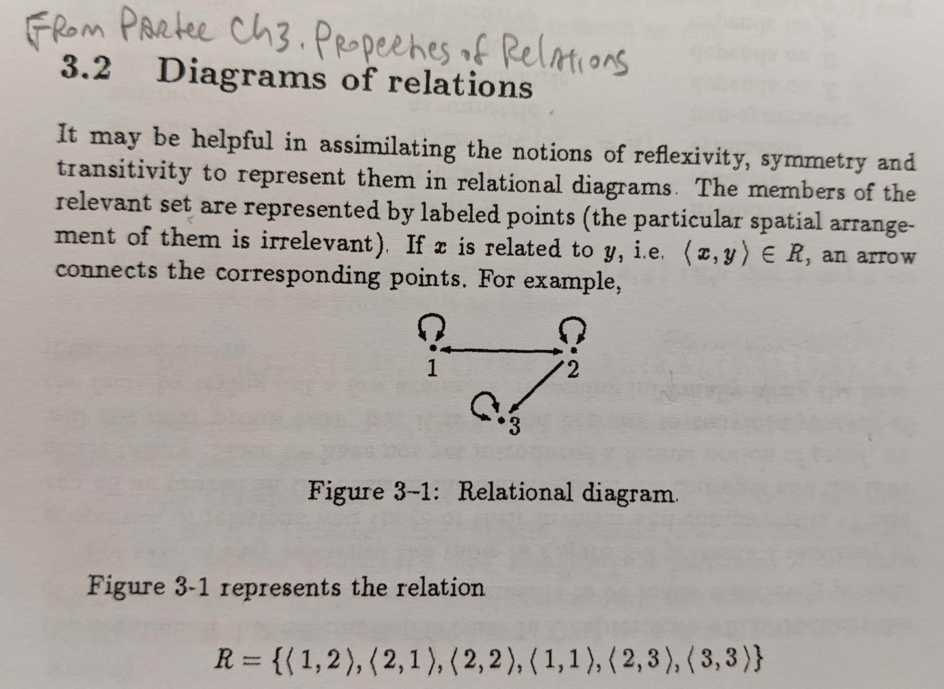
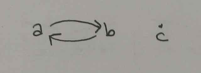
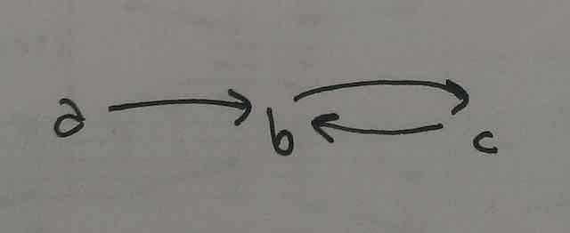
In ordinary graphs, it is usually forbidden for an edge to join any vertex to itself. For some applications, though, it is useful to allow graphs that permit that. When such edges are allowed, they are called self-loops or just loops (and sometimes the graphs that include them are called pseudographs). Some examples where those are allowed are in the “next-state diagrams” for formal automata, that we’ll look at in later classes. Also when using digraphs to represent relations, as Partee does in a reading we looked at:
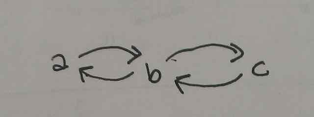
In ordinary graphs, it is usually forbidden for more than one edge to join two vertices (in the same direction: a digraph like the one shown earlier is allowed to have a directed edge from c to d, and then another directed edge from d to c). For some applications, though, it is useful to allow graphs with multiple edges between some pairs of vertices. (Sometimes these are called multigraphs. The famous Bridges of Koenigsberg problem, which launched the discipline of graph theory, makes use of undirected multigraphs rather than ordinary ugraphs.)
As is implicit in the above explanations, a graph can have many vertices but no edges at all. Or it may have edges connecting some proper subsets of its vertices, but have several disconnected “pieces.” We’ll introduce some terminology to describe this more carefully below.
(In some applications, it is permitted for there to be edges that “hang free,” instead of always joining a pair of vertices. They lack a vertex on one of their ends, sometimes even on both ends. We won’t be discussing graphlike structures of this sort, though.)
Here’s some additional terminology for reference, but you probably won’t need to use this unless you’re getting more into the mathematics of graphs than we will:
Consider a ugraph, and let a walk be a sequence of adjacent vertices, perhaps visiting the same vertex several times, perhaps even traversing the same edge several times. There is further terminology for different restrictions on this notion.
A trail is a walk of 1 or more vertices, where (as in any walk) successive vertices in the sequence are adjacent, and (now we impose special restrictions) no edge is traversed more than once. In trails, vertices are allowed to be revisited.
A path is a walk of 1 or more vertices, where no vertex (and thus no edge) is visited more than once, with the exception that the ending vertex is allowed to be (but needn’t be) identical to the starting vertex. (You’re much more likely to encounter this vocabulary than the more general notions of a trail or walk.) A closed path, where the start and end vertices are the same (and the path traverses at least one edge), is called a cycle. A path of length 0 would just be a single vertex. Any single edge would give us a path of length 1. Paths of length 2 would include 2 edges; and so on.
Recall the notion of a self-loop, discussed before. If those are allowed, they would count as cycles (on our definitions). They would be cycles of length 1. But there can be longer cycles too. In an ordinary ugraph, where (as opposed to a multigraph) at most a single edge joins any two vertices, the shortest cycle which isn’t a self-loop would have length 3. Although it’s common to prohibit self-loops from the graphs one is talking about, it’s common to allow longer cycles. For some purposes, though, it is useful to prohibit cycles too, and only consider acyclic graphs.
In the above example, there are paths of length 0 and 3 from each vertex to itself. (Only the latter paths are called cycles.) There’s also a path of length 1 from b to b because of the self-loop (if that’s allowed, and this is also counted as a cycle). The walk that goes from a to b and then over the self-loop again to b and then to c would not satisfy the definition of a path.
Some trails and paths have special names, though again these aren’t terms you’re likely to encounter. They’re provided here for reference.
The components of a ugraph are the maximal subsets of vertices such that for every pair in the set, there is a path between them; together with all the edges joining those vertices. When a graph has only one component — that is, when there’s a path between any two vertices in the graph — then the graph is called connected. (The notion of a graph’s being complete, mentioned earlier, is more demanding: that requires that there be not just a path, but more specifically an edge, between any two vertices.)
Some more terminology about connectedness and components, again just for reference:
A component of a graph is an example of a more general notion, that of a subgraph. A subgraph of a graph G would be given by any subset of G’s vertices, joined by some subset of the edges that join those vertices in G. G’s components are its maximal connected subgraphs: that is, subgraphs of G that are connected and aren’t proper subgraphs of any other connected subgraphs of G.
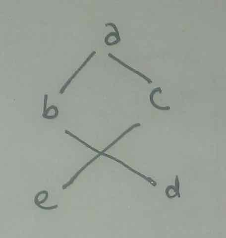
Here’s an example we saw before of a ugraph. It has two components:
Here’s another ugraph with two components:
In the second graph, the one component is the subgraph  and the other is the subgraph
  .
.
We should think of a graph G in a way that’s independent of any specific choices about the identities of its vertices.
Mathematically, a graph is just a pattern by which any set of n-many vertices may be joined. But in elementary expositions, graphs are often presented as constructions where the vertices do have some specific identity. Then, when we consider the question whether graph H is a subgraph of G, or whether it is equivalent to G, we have to ignore the specific identities of those vertices. We count graphs as equivalent so long as there is some isomorphism between them that preserves the relevant edge structure. And for H to count as a subgraph of G, it doesn’t have to contain any of the same specific vertices as G does; it’s enough that there is a homomorphism from G to H that preserves the relevant edge structure. (We will explain these “-morpishm” notions in later classes.)
A philosophically more satisfying way to proceed would be to work with a more abstract understanding of graphs, where the vertices never acquire a specific identity in the first place. There are ways to do this, but they are not how graphs are usually presented in elementary expositions.
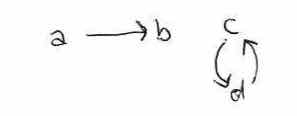
When it comes to digraphs, there are several different notions of connectedness. It’s clear that a digraph like this one is unconnected, in every sense:
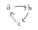
On the other extreme, it’s clear that a digraph like this one is connected, in the most robust sense. Every pair of vertices is joined by a path (in both directions, in this example), which always travels “with” the direction the digraph’s arrows. This is called a strongly connected digraph.
This is also strongly connected:
More terminology: when we can assign directions to the edges of some ugraph, in a way that results in a strongly connected digraph, we say that the original ugraph is orientable.
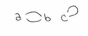
Between the extremes just displayed, there are different kinds of digraphs that are kind-of, sort-of, in-a-way connected. For example, in this digraph:
for any pair of vertices you choose, you can always find a path that travels “with” the direction of the digraph’s arrows, but sometimes this path will only go from the second vertex to the first, and not from the first to the second. There is a path of this sort from a to c, but not one from c to a. (This is sometimes called being unilaterally connected.)
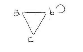
The following two digraphs are connected in an even weaker sense:
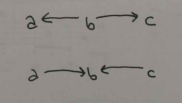
In these cases we cannot find a path that travels only “with” the direction of the arrows either from a to c or from c to a. Unlike digraph #2, though, at least in this case there is a kind of path between a and c. It just requires sometimes traveling “with” the direction of an arrow, and sometimes traveling “against” it. (We can call these semipaths; and digraphs of this sort are sometimes called weakly connected.)
These are all legitimate notions of connectedness and of directed paths. But henceforth, when I speak of a directed path from c to a, I shall mean only the kind of structure we see in digraphs #3 and #4.
There are natural correlations between (non-multi)graphs and finite relations. One way to think of this would associate the holding of the relation with the presence of an edge. Then, when we have a ordinary graph that excludes self-loops, the relation would have to be irreflexive. When the relation is symmetric, we could think of it as correponding to either an ugraph, or to a digraph that just happens to also have a reverse arrow wherever it has an arrow. When the relation is not symmetric, we should understand the graph to be directed.
A different way to correlate graphs and relations would associate the holding of a relation not with the presence of an edge but the presence of a path. This makes sense when the relation is reflexive and transitive. Then the relation holds between v₁ and itself iff there’s a path starting with v₁ and ending with v₁ — and there always is such a path, of length 0. (We wouldn’t need to require “self-loopy” paths of length 1.) It holds between v₁ and v₂ if there’s a (directed) edge joining v₁ to v₂, or a (directed) edge joining v₁ to … to v₂. If the relation fails to be symmetric, we should here also understand the graph to be directed.
The presence or absence of an edge between two vertices carries “a single bit” of information about how those vertices are related. Sometimes we want to use graphs to represent richer information. For example, we might be using the vertices to represent cities, and want to associate with the edges information about how much it costs to travel between those cities. We can do this by just adding to our graph a function from edges into whatever kind of information we want to work with.
Graphs with labeled edges of this sort, especially when the labels are real numbers, are sometimes called networks.
As I mentioned before with the two train lines going through Market Street Terminal, for some purposes, we might also (or instead) want to have labels for vertices. That example already gave us a case where we might want to have one object simultaneously occupy multiple vertices/positions in a graph. The vertices, on the other hand, are the positions. Their numerical sameness and difference is what constitutes sameness and difference of graph positions. It would make no sense to have two positions (which might, or might not, have different incident edges) constituted by what is numerically just a single object. That’s why we can’t (in general) let the labels (train stations) be the vertices. The labels are instead assigned to the vertices, and depending on our application we can allow or forbid one and the same object labeling several vertices.
Here’s another example where we might want to allow that.
Suppose we are making a syntax tree of a sentence where the same word appears multiple times. A syntax tree is a kind of graph, which we’ll look at more closely in a moment. So now if we think that what gets associated with the vertices of this graph are the word-types of the relevant sentence, this would be a case where we’d want to associate the same object (a given word-type) with multiple vertices.
You might protest: why don’t we understand these trees as inhabited by word tokens instead of word types? Then we can be sure that when “the same” word appears multiple times in the sentence, there will always be multiple tokens. So we can let those tokens just be the vertices, rather than making them label some separate set of vertices.
Nice try, but that strategy will not work in general. Consider the following inscription of the sentence-type "stupid is as stupid does":
| stupid | is as does. |
Or this inscription of the sentence "If it was stupid to date John once, it was more stupid to date him twice":
If it was | stupid | to date John once, to date him twice. |
Given the most natural understanding of the notion of a token, these inscriptions each contain only a single token of the word-type "stupid". Yet that word should occupy two different syntactic positions in each sentence. Some philosophers will respond to this by distinguishing what I’m here calling a token, and what we might call an occurrence. Even if the above inscriptions have only one token of the word-type "stupid", they’d say, that word-type nonetheless has two occurrences in the sentence. (Some philosophers even insist that that’s what they mean by “token.” This surprises me, but ok.)
I have no objection to this notion of an occurrence. But this occurrence-talk is just another way of expressing the idea of a single word-type being associated with distinct syntactic positions. The two occurrences aren’t given to us in advance, in such a way that we could use them to build the two positions or vertices. The distinctness of the occurrences instead already assumes the distinctness of the positions. And that’s just what I’m recommending. We should think of the words — it could just be the word-types, there’s no need to invoke tokens here — as labeling distinct vertices or positions in the syntax tree. There is no obstacle to one and the same word labeling multiple vertices, because the label doesn’t constitute the vertex, it’s just assigned to it.
There are three different routes for getting from the ideas we’ve reviewed so far to the notion of a tree.
One route starts from the notion of a ordinary ugraph. Any ugraph without cycles can be called a forest, and a connected forest — that is, a forest with just one component — can be regarded as a tree. In such ugraphs (and only in them), there will be exactly one path between each pair of vertices. Any of the vertices can then be chosen to play the special role of the tree’s root, and the selection of the root will impose an ordering on the rest of the vertices, tracking the directions towards / away from the root. For example, in the following ugraph:
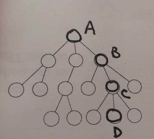
as I said, any of the vertices could be selected as the root, but if we select A as the root, then relative to vertex C, B will be closer to the root and D will be farther away. Any vertices of degree 1 (that aren’t themselves the root) are called the leaves of the tree. Vertices that aren’t the root and aren’t leaves are called interior vertices.
(Any tree with n vertices will have exactly n-1 edges. Any ugraph with n vertices and fewer than n-1 edges must be unconnected; if such a graph has n-1 edges and happens to be connected, then it must be a tree.)
A different route wouldn’t impose an order onto a tree by designating a root, but would instead start with digraphs that already have an order. Not every digraph could constitute a tree, but for those that do, the root would just be the vertex that doesn’t have any incoming arrows.
(Here is how to specify the eligible digraphs: they are acyclic, and at least weakly connected in the sense illustrated in the digraphs #6 diagram, above, and every vertex has at most 1 incoming arrow. Then there will be a unique vertex with no incoming arrows, and it counts as the root.)
A third route for getting a tree will be described later.
Given a tree-like structure via one route or another, we can say that one vertex dominates another vertex if there is a path leading from the second, through the first, going towards the root of the tree. (We also count vertices as dominating themselves.) Here’s an example:
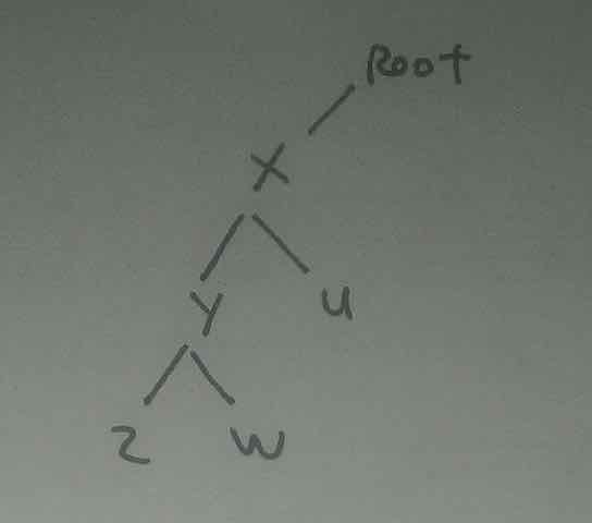
In this tree the vertex x dominates all of the following vertices: x, y, z, w, and u. The dominating relation is reflexive, transitive and anti-symmetric, and thus counts as a non-strict partial order. To help fix ideas, another example of a relation of that sort is the ⊆ relation on sets.
The root vertex in a tree is not dominated by any vertex but itself. The leaf vertices in a tree do not dominate any vertex but themselves.
When we diagram a tree on paper, the diagram may end up having geometrical properties that aren’t any part of the mathematical structure we’re diagramming, but are just artifacts of our particular drawing. For example, the right-left relations in graphs we diagram generally are just accidents of our drawing. But one can if one wishes impose an ordering on the edges leaving each vertex. When using trees to represent syntactic structures, we do in fact do this. We call this ordering preceding, and by convention we will respect it in the left-right structure of the tree diagrams we draw. So if the tree #2 diagram above is understood to have its edges ordered in this way, then we’ll say that vertex y precedes vertex u, and vertex z precedes vertex w. It is useful to think of “child” vertices as inheriting the precedence relations of their parents, so that we can say that vertices z and w both precede vertex u as well. We will want to rule out cases like this:
We can do that by saying that if b precedes c then all nodes dominated by b have to precede all nodes dominated by c.
Whereas a good model for the dominating relation is ⊆, the precedence relation is instead usually thought of like the proper subset relation (⊂). We don’t allow vertices to precede themselves.
We’ve described how a dominating relation can be read off of a rooted tree, and how a precedence relation can be added to such a tree. A different way to go is to take the dominating relation and the precedence relation as given, and to let the tree in question be implicitly specified by them. For example, this is how Partee, ter Meulen, and Wall introduce constituent structure trees in section 16.3 of their Mathematical Models in Linguistics. (This is what I earlier called a “third route” for getting a tree.)
However we get to a tree with a dominating and precedence structure, we define the fringe or yield of a labeled tree to be the sequence of labels assigned to the tree’s leaves, in their left-to-right precedence order. So if we have a tree:
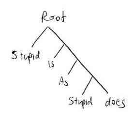
where its leaves are understood to be labeled by the indicated English words, its fringe would be the sequence "stupid", "is", "as", "stupid", "does".
This tree would have the same fringe:
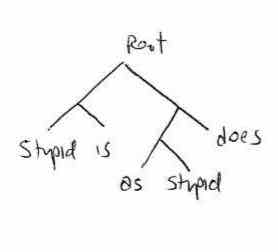
but it’s a different tree, because of its different structure.